A curve
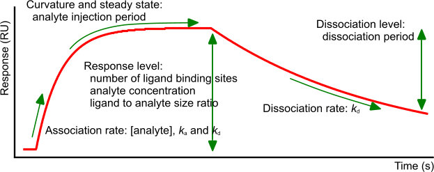
Let us look at a single exponential curve. The example sensorgram consists of an association, steady state and dissociation phase. What is important in the different parts of an interaction curve?
Association: At the injection start of the analyte, the transition between flow buffer and analyte, known as the bulk shift, should be small and proportional to the analyte concentration. The bulk shift originates from the (refractive index) differences between the flow buffer and the sample buffer. The initial part of the curve should not be a straight line, which indicates a mass transport free interaction (see below). The association should follow a single exponential and have at least some curvature before the analyte injection ends (1),(2). The speed of complex formation depends on the association rate constant, the analyte concentration and the number of free ligand sites.
Steady state: When the analyte injection time is long enough, the curve should level out, indicating that the number of association events is equal to the number of dissociation events. The curve should be horizontal! Although not strictly correct, this situation is often referred to as equilibrium. The response at steady state (equilibrium) is denoted Req and is dependent on the number of ligand binding sites, the analyte concentration and the equilibrium dissociation constant. A slow dissociation rate will require a long injection period to reach steady state. When the dissociation is fast (kd< 5.10-2), steady state is reached quickly upon analyte injection. The Req can be calculated with the following equation.

Dissociation: During the dissociation, the curve should follow a single exponential. The dissociation is only dependent on the dissociation rate constant but in cases of a strong interaction, the curve can be almost horizontal. To analyse a slow dissociation, the dissociation period should be long enough to have at least 5% signal decrease compared to the initial response (3). However, even a slow dissociation curve should level out to the value of the baseline at the beginning of the interaction. When there is a residual response after the dissociation, this can be an indication of non-specific interaction with the matrix. To force the analyte from the ligand or matrix, an injection with a low pH or high salt solution can be done providing that the ligands will stay intact.
Curve dependencies
Although the 1:1 interaction is a single exponential, the shape can vary a lot depending on the values of the parameters. The overall shape of the curve can be deduced from the kintic and is determined by the analyte concentration, association rate and dissociation rate constants. The number of ligand binding sites and the relative size differences between the ligand and analyte determine the level of response. In addition, the analyte injection time and the dissociation time determine what portion of the interaction curve is recorded.
Equilibrium and saturation
There is a distinct difference between the response at equilibrium (steady state) and at ligand saturation. When the interaction time is long enough, the binding response levels out and is said to have reached equilibrium. At this point, the number of newly formed complexes equals the number of complexes breaking up. However, when a higher analyte concentration is injected, a new equilibrium is reached with a higher response. The analyte concentration can be raised even further until all the ligand binding sites are occupied and the maximal response is reached. Nevertheless, at full ligand saturation the interaction is at equilibrium because complexes are formed and breaking up. Thus, while a response that reaches saturation will be at equilibrium, an equilibrium response may not be at saturation (2).
If the analyte concentration is expressed in equivalents of the KD some new insights follow (see figure ‘Saturation’).
- Even at low concentrations, the curve will reach steady state. At a low analyte concentration, the time to reach equilibrium will be longer than at high analyte concentrations.
- When the analyte concentration equals the KD, the response is half-maximal.
- You need at least 10 times the KD in analyte concentration to reach 90% of the Rmax.
- To reach the true Rmax, a very high analyte concentration is needed. Luckily, it is not necessary to saturate the ligand to get meaningful results. Curve fitting programs can extrapolate the data to calculate the Rmax. To obtain reliable results, the analyte concentration range should be wide enough to give between 20% and 80% ligand saturation (e.g. 0.1 – 10 times the KD).
Rmax
The response upon analyte binding is dependent on the number of ligand molecules immobilized and the size of the ligand and analyte (ligand - analyte molecular size ratio). Furthermore, the response is dependent on the number of interaction sites of both ligand and analyte. When all ligand binding sites are occupied by the analyte, the maximal response (Rmax) is reached.
Rmax is dependent on the surface capacity of the ligand and the molecular mass of the analyte. The rate constants ka, kd and the equilibrium constant KD is independent of the concentration of both analyte and ligand but is dependent on the pH, salt, temperature and pressure of the solution. Therefore, it is important to keep the experimental conditions constant and to mention these in your publication.
The shape of the curves is highly dependent on the dissociation rate constant. In the figure are five dissociation rates (10-1 – 10-5 s-1) with the same association rate (105 M-1s-1) and an analyte concentration of 1 times KD. The curve with the fastest dissociation rate will reach steady state much quicker compared to the other. Can you figure out which curve has the fastest dissociation rate?
The time to reach equilibrium can be calculated using Eq. 2. Theta (Θ) denotes the fraction of equilibrium. For instance, to reach 95% equilibrium, Θ = 0.95.

To reach steady state quicker it is possible to raise the analyte concentration, but this will not always work. Analyte concentrations above 100 times KD often give binding curves which are not an exponential. It is better to increase the injection time. However, as the table shows, this can be a very long injection period and is mainly dependent on the dissociation rate constant.
| concentration analyte | kd (s-1) | |||
|---|---|---|---|---|
| 10-1 | 10-2 | 10-3 | 10-4 | |
| 0.01 x KD | 68 s | 11.5 min | 115 min | 1140 min |
| 0.1 x KD | 63 s | 10.5 min | 105 min | 1047 min |
| 1 x KD | 34 s | 5.8 min | 57 min | 576 min |
| 10 x KD | 6 s | 1 min | 10.5 min | 1105 min |
| 100 x KD | 1 s | 0.1 min | 1 min | 11 min |
| ka = 1.105 M-1s-1 | ||||
Equilibrium analysis
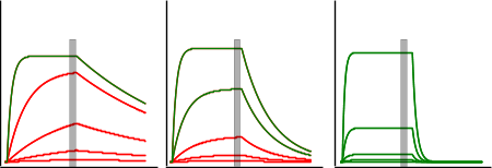
One of the most common mistakes is to use equilibrium analysis on curves which are not in equilibrium (steady state) (2). Equilibrium is reached when the number of associations equals the number of dissociations and consequently the response level remains constant!
The figure ‘Equilibrium analysis’ shows three sensorgrams of which only C can be used for equilibrium analysis because there all the green coloured curves level out before the end of the injection. This is important, because only at equilibrium the response of the complex is directly proportional to the concentration of the analyte. And only with the response at equilibrium a reliable dissociation constant can be determined.
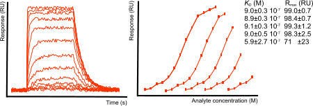
For equilibrium analysis, it is not necessary to saturate the ligand as long as the equilibrium curve has enough curvature to be fit properly. In the next figure, subsequent points are left out in the analysis. For a reliable result, roughly 30 to 40 percent of the ligand must the saturated.
Analyte concentration range
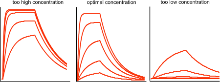
The concentration range of the injected analyte is important. With too high concentrations, the curves tend to bunch together in the upper part of the sensorgram. Too low concentrations will give low responses and little curvature. The best concentration range is somewhere around 0.1 – 10 times the KD of the interaction. This will space the curves evenly over the sensorgram, having high and low responses. This requires knowledge of the kinetics. The best approach is to start with a low concentration, for instance 10 nM and work your way up until you obtain nice curves. When you have established the concentration range, design an experiment with a dilution series. It is better to use a dilution series because they are easier to make and problems with the injections are more quickly detected. Try to make a dilution series covering the 0.1 x KD to 10 x KD. Add repeats of the dilutions to show the system is stable. Use a minumum of five analyte concentrations and repeat at least one twice.
The figure below shows sensorgrams with a) too high, b) optimal concentration and c) too low concentration of analyte. Thus, these sensorgrams clearly show the required (optimal) concentration of analyte to be used.
It is possible to obtain kinetics from a single analyte concentration but generally it is better to use multiple concentrations to determine the kinetic rate constants. This is because global analysis over several curves will constrain the kinetic parameters better (especially the Rmax). In some cases when fitting one curve the fitting looks ok but the Rmax can be fairly off which can indicate that also the kinetic rate constants can be off. With three or more curves covering a wide analyte concentration range the fit will be more reliable.
As said, when the injection time of the analyte is long enough, the association rate will equal the dissociation rate and the curve will reach steady state. The time to reach steady state depends greatly on the dissociation rate constant and the analyte concentration. In principle, you don’t need all curves in steady state to get meaningful results, but you should have enough curvature in the curves.
Curve response
The response of the sensorgram should match the amount of immobilized ligand and the concentration of analyte used. Because you know which ligand and analyte is used, you can calculate the theoretical Rmax with:

Although a valid formula, in general it is not practical because the fraction active ligand is unknown. Depending on the immobilization technique used, only a larger or smaller fraction is still biological active.
As an alternative, the Rmax can be determined by saturating the ligand by injecting high analyte concentrations. However, this is not always possible (see above at steady state). Luckily, it is not important to know the Rmaxsub> to get meaningful kinetic results.
In the fitting procedure, the Rmax is determined as one of the parameters. As long as the calculated Rmax is in agreement with the measured values, full saturation of the ligand is not necessary.
In addition, high analyte concentrations and the following high responses tend to have problematic kinetic behaviour. So keep in mind that sensorgrams with a low response level (< 100 RU) are better than curves with a high response.
What about these fast on and of curves? Are they real or is it bulk effect?
When it is real kinetics, the shape of the curves is almost totally determined by the dissociation rate. Because of the fast dissociation, the curves reach equilibrium almost directly. The height of the response is directly proportional to the analyte concentration. With increasing analyte concentration, the surface will saturate as opposed to other effects like high salt or non-specific binding.
Real kinetics can thus saturate the ligand at high analyte concentrations. If the response keeps getting higher, other effects such as non-specific binding, bulk refractive distortion causes these high responses.
References
| (1) | Rich, R. L. and D. G. Myszka - A survey of the year 2002 commercial optical biosensor literature. J.Mol.Recognit. 16: 351-382; (2003). Goto reference |
| (2) | Rich, R. L. and D. G. Myszka - Survey of the year 2007 commercial optical biosensor literature. J.Mol.Recognit. 21: 355-400; (2008). Goto reference |
| (3) | Katsamba, P. S., I. Navratilova, M. Calderon-Cacia, et al. - Kinetic analysis of a high-affinity antibody/antigen interaction performed by multiple Biacore users. Analytical Biochemistry 352: 208-221; (2006). |
| (4) | BIACORE AB - BIACORE Technology Handbook. (1998). |
SPR pages book
For a more thorough explanantion of the exponential curve, sensorgrams and curve fitting, take a look at the SPRpages book.