Reporting results
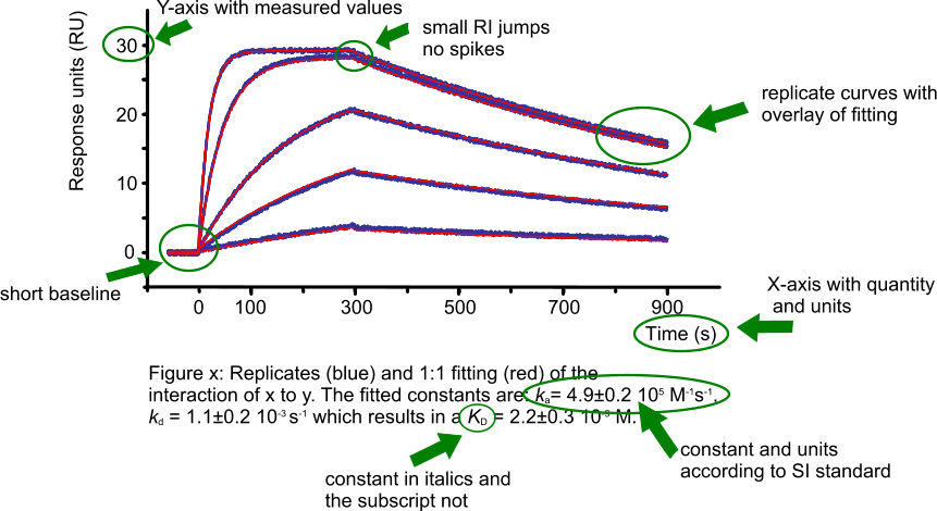
When reporting your results, always show the curves and the overlay of the fitting (1). One figure gives more insight than a hundred words. Just reporting a KD value is insufficient and leaves the reader in doubt as to whether the fitting is following the curves properly. Only the curves and the overlaid fitting will convince the reader of the quality of the experiment and the fitting (2).
Global fitting gives only one value (and standard error) per parameter per data set. By running replicate experiments, more values per parameter are obtained. This is the correct way to obtain statistics, even if local fittings are used. Separate curves in a sensorgram with a concentration series should not be treated as replicates for statistical purposes; they are part of a single data set (3).
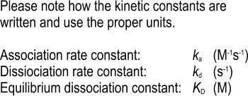
Report both association and dissociation rate constants (ka, kd) and the equilibrium dissociation constant (KD). By reporting all three values the reader can verify the KD and deduce if it was due to a high ka or a low kd (or both; see affinity plot).
Make sure to round the values and associated errors to the first significant digit. Instead of reporting ka = 4.32 ± 0.17 105 M-1s-1, report ka = 4.3 ± 0.2 105 M-1s-1. For more information on reporting values read for instance Wikipedia (4).
Report the calculated values with care. Do not overestimate the precision of the analysis. In general, the equipment used has upper and lower limits to the values that can be accurately determined (5). In addition, analyte concentration errors have a direct influence on the ka and therefore on the KD.
Publishing a sensorgram
When adding a sensorgram to your publication, the figure should not only be simple and clear to understand (2) but must also contain all the information so the reader can be confident that the experiments are well performed and analysed. The next figure shows an example of a sensorgram with fitting, highlighting the important parts of the figure.
Describing a biosensor experiment
Equal important to the method you have used in the experiments, is what you report afterwards in your publication. You already know that it is very hard to repeat a published experiment. This is mainly because the author is not writing down all the experimental conditions. This shortcoming is recognised and David Myszka proposed the TBMRFAADOBE (The Bare Minimum Requirements For An Article Describing Optical Biosensor Experiments) (1).
- instrument used in analysis
- identity, source, molecular weight of ligand and analyte
- surface type
- immobilization condition
- ligand density
- experimental buffers
- experimental temperatures
- analyte concentrations
- regeneration condition
- figure of binding responses with fit
- overlay of replicate analyses
- model used to fit the data
- binding constants with standard errors
Example text
As an example, here is a possible text for the methods part of your publication
The surface plasmon resonance experiments were performed using a [instrument] equipped with a [type] sensor chip. The ligand (60 kDa, >90% pure based on SDS–PAGE) was immobilized using amine-coupling chemistry. The surfaces of flow cells one and two were activated for 7 min with a 1:1 mixture of 0.1 M NHS (N-hydroxysuccinimide) and 0.4 M EDC (3-(N,N-dimethylamino) propyl-N-ethylcarbodiimide) at a flow rate of 5 μl/min. The ligand at a concentration of 5 μg/ml in 10 mM sodium acetate, pH 5.0, was immobilized at a density of 200 RU on flow cell 2 and flow cell 1 was left blank to serve as a reference surface. Both surfaces were blocked with a 7 min injection of 1 M ethanolamine, pH 8.0. To collect kinetic binding data, the analyte (34 kDa, >95% pure based on SDS–PAGE) in 10 mM HEPES, 150 mM NaCl, 0.005% P20, pH 7.4, was injected over the two flow cells at concentrations of 90, 30, 10, 3.3 and 1.1 nM at a flow rate of 60 μl/min and at a temperature of 25°C. The complex was allowed to associate and dissociate for 90 and 300 s, respectively. The surfaces were regenerated with a 5 s injection of 10 mM H3PO4. Triplicate injections (in random order) of each sample and a buffer blank were flowed over the two surfaces. Data were collected at a rate of 1 Hz. The data were fit to a simple 1:1 interaction model using the global data analysis option available within [software name] software.
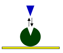
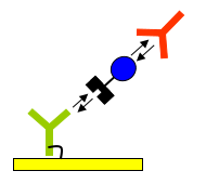
Cartoons
As an additional service to your readers, you can incorporate a figure depicting the layout of your interaction.
References
| (1) | Rich, R. L. and D. G. Myszka - Survey of the year 2007 commercial optical biosensor literature. J.Mol.Recognit. 21: 355-400; (2008). Goto reference |
| (2) | Rich, R. L. and D. G. Myszka - Grading the commercial optical biosensor literature-Class of 2008: 'The Mighty Binders'. J.Mol.Recognit. 23: 1-64; (2010). Goto reference |
| (3) | Biacore AB - Information about BiaEvaluation 3.0. (2000). |
| (4) | Wikipedia - International System of Units. (2022). Goto reference |
| (5) | Yau, K. Y., M. A. Groves, S. Li, et al. - Selection of hapten-specific single-domain antibodies from a non-immunized llama ribosome display library. Journal of Immunological Methods 281: 161-175; (2003). |