Steady state
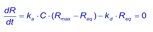
When the pulse of analyte continues long enough for the binding to reach steady state, the net rate of binding dR/dt is zero. Since the analyte is continuously added and removed from the system by sample flow, the situation is steady state rather than equilibrium according to the strict definition of the terms (1).
Equilibrium constants are determined by measuring the concentration of free interactants and the complex at equilibrium.
Equilibrium constants are denoted by upper case K. Using KA for the association quilibrium constant (M-1) and the KD for the dissociation equilibrium constant (M). The association equilibrium constant is the inverse of the dissociation equilibrium constant. The looser term "affinity constant" should be avoided when possible (1).

KD describes the system at equilibrium but not the dynamics. For the dynamics, refer to the association and dissociation rate constants (2). The best parameter to compare the strength of the binding is the dissociation rate constant (kd) because this parameter gives the time an interaction exists.
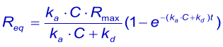
At equilibrium, the concentration of the complex is directly proportional to the response (Req) and the concentration of the analyte is the concentration injected (C). The concentration free ligand (Rmax - Req) can be derived from the complex if the total surface binding capacity (Rmax) is known. The association equation can be written as:
Equilibrium constants are determined with great sensitivity if the analyte concentration is equal to the dissociation constant KD that gives 50% saturation of the surface. If pilot experiments reveal that the equilibrium surface saturation is outside the range 20—80%, adjust the analyte concentration accordingly for the best results. Use a low flow rate (2—5 µl/min) if longer injection times are required (5).
Equilibrium measurements are unaffected by mass transport and analyte rebinding (4). This makes it possible to use high ligand concentrations and low flow rates.
Time to reach equilibrium
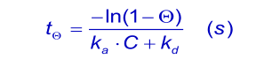
An important experimental consideration is the time taken to reach equilibrium. From the integrated rate equation for association the time required (Rθ) to reach a fraction of equilibrium (θ = R/Req) can be derived as:
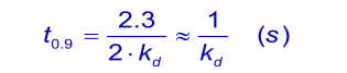
When the analyte concentration is equal to the dissociation constant KD ( kd/ka), the time taken to reach 90% of equilibrium (θ = 0.9) is given by:
Sometimes, the normal injection times are too short to reach equilibrium. It is then possible to add the analyte to the running buffer (6). Initially a low concentration analyte is used and after equilibrium raised to the next higher concentration. After that, the whole is reversed to show that the binding is reversible.
| Conc. analyte | kd (s-1) | |||
| 10-1 | 10-2 | 10-3 | 10-4 | |
| 0.01 x KD | 68 s | 11.5 min | 115 min | - |
| 0.1 x KD | 63 s | 10.5 min | 105 min | - |
| 1 x KD | 34 s | 6 min | 67 min | 9.6 hour |
| 10 x KD | - | 63 s | 10.5 min | 105 min |
| 100 x KD | - | - | 68 s | 11 min |
References
| (1) | BIACORE AB BIACORE Technology Handbook. (1998). |
| (2) | BIACORE AB Kinetic and affinity analysis using BIA - Level 1. (1997). |
| (3) | Kortt, A. A. et al Analysis of the binding of the Fab fragment of monoclonal antibody NC10 to influenza virus N9 neuraminidase from tern and whale using the BIAcore biosensor: effect of immobilization level and flow rate on kinetic analysis. Anal.Biochem. 273: 133-141; (1999). |
| (4) | van der Merwe, P. A. Surface Plasmon Resonance. PDF file from internet (2003). |
| (5) | BIACORE AB BIACORE Application Handbook. (1998). |
| (6) | Myszka, D. G. et al Equilibrium analysis of high affinity interactions using BIACORE. Anal.Biochem. 265: 326-330; (1998). |