SPR is not an Art!
Surface Plasmon Resonance (SPR) seems to be difficult for many people. Judging on the literature (1),(2) many of you are struggling to get nice sensorgrams with easy to fit curves. However, SPR is straightforward when you know what you are doing. Consequently, you have to learn how SPR works, how to perform an experiment and how to analyze it. So what are the key parts of a proper SPR experiment?
Start with the best ingredients. That is a clean machine (3), high quality reagents, pure ligands and analytes. Filtered and degassed flow buffer and a well-equilibrated instrument will minimize drift, shifts and air spikes during the experiments. Use pure well-defined ligands on the sensor chip surface. Match the buffer of the analyte to the flow buffer to minimize bulk shifts due to buffer differences.
Optimizing immobilization
Immobilize a low amount of ligand. It is hard to give absolute numbers, because this depends on the ligand and analyte combination. Therefore, the immobilization steps needs optimization. Begin with calculating the theoretical amount of ligand you need to get 100 RU’s of analyte binding. Immobilize the ligand and equilibrate the surface. Check the response with a series of analyte injection from a very low concentration to a high concentration. Observe the shape of the curve (association and dissociation) and the height of the response. From the height of the curve, you can estimate the amount of ligand that is still kinetically active. If necessary, recalculate the amount of ligand to be immobilized and make a new surface. Use the lowest amount of ligand still giving a proper response value.
In addition, the first analyte injections will give you valuable information about the interaction kinetics. Has the association curvature? Is mass transport absent? Is the dissociation slow or fast? The answers will guide you in the design of the following experiments. Depending on the first results, you can choose the best injection strategy to use.
Injection strategies
The multi cycle kinetics is the most common way to perform experiments. It is useful for most of the interactions except the very strong. Each injection of analyte or blank is done in a separate cycle. At the end of the experiment, all the single curves are put together in one sensorgram for analysis. By running single injections in an automated method, the overlay of all the cycles is very easy.
The kinetic titration (or single cycle kinetics) is useful with interactions which are difficult to regenerate or when regeneration is detrimental to the ligand (4). The analyte is injected from a low to high concentration with short dissociation times in between and a long dissociation time at the end (not shown here). All the injections are analysed in one sensorgram with a special equation for kinetic titration. The models often limit the kinetic titration to five analyte injections. The kinetic titration is also useful in finding the optimal analyte concentration. Start with a low analyte concentration and increase the analyte concentration each new injection at least five fold until a proper signal is obtained.
The 'short and long' experiments are done when the dissociation is very slow. Injections with low analyte concentrations take a long time to dissociate sufficient to be analysed. Therefore, to obtain adequate decrease in response, only the highest analyte concentration is used for a long dissociation time. The lower analyte injections are regenerated after a short dissociation period. This will greatly speed up the experiment.
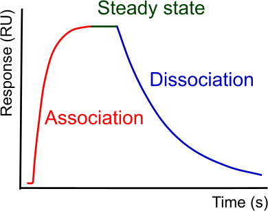
Steady state experiments are possible when the dissociation rate is sufficiently fast. In general when the kd is faster than 10-3 s-1. With a slow dissociation rate, it takes too long to reach steady state within one analyte injection volume (depending on the type of instrument). A steady state experiment is often used with small compounds, which have a fast dissociation and therefore reach steady state quickly. When steady state is reached very fast, the association and dissociation rate are hard to determine. In addition, a steady state experiment is frequently used to confirm the dissociation constant.
Experiments
Perform the first experiments with five analyte injections within a concentration range between 0.1 and 10 times the expected KD of the interaction. Add some blanks for double referencing. After the first experiments, you have to judge if the curves are up to standard. Ask yourself the following questions.
- is mass transport absent?
- is the analyte concentration range ok?
- is reference channel performing well?
- is the calculated Rmax within the expected range?
- is the sensorgram following a 1:1 model?
If you can all answer all questions with yes, then you are on the right path. If not, first optimize the interaction before you try to extract any meaningful results from these low-quality curves.
Sensorgram analysis
The analysis of the sensorgrams is not difficult when the curves are nice and clean and following a 1:1 interaction. The fitting will follow the curves nicely and the results are unambiguous. However, this is not always the case.
So before using other fitting models than the 1:1 Langmuir model make sure that:
- the system is clean and equilibrated
- the ligand is pure and homogenous
- the amount of ligand is low to minimize mass transport
- the analyte is pure and homogenous
- the analyte concentration range is wide enough (0.1 – 10 x KD)
- the analyte buffer is matching the flow buffer minimizing bulk shift
- the injection time is long enough to give the association curvat the dissociation is long enough to give a reasonable signal decay
- the reference channel is performing well
- blank injections are used for double referencing
- replicate analyte injections are done to prove the system stability
In the situation that, after optimization, the single exponential model does not fit, one can choose an alternative model. For instance, when an intact antibody is used as an analyte, bivalency must be taken in to account (5),(6). Every time when another model than a single exponential is chosen, the binding mechanism should be confirmed by other means of detection.
Conclusion
SPR in not an Art! It is science and therefore takes some effort to understand and perform. This article gives you a brief overview what to look for and what to learn. Browse the sprpages for more information or buy the sprpages book with the information of the website and more in-depth explanations, procedures, tips and tricks.
References
| (1) | Rich, R. L. and D. G. Myszka - Survey of the year 2007 commercial optical biosensor literature. J.Mol.Recognit. 21: 355-400; (2008). Goto reference |
| (2) | Rich, R. L. and D. G. Myszka - Grading the commercial optical biosensor literature-Class of 2008: 'The Mighty Binders'. J.Mol.Recognit. 23: 1-64; (2010). Goto reference |
| (3) | Navratilova, I., G. A. Papalia, R. L. Rich, et al. - Thermodynamic benchmark study using Biacore technology. Analytical Biochemistry 364: 67-77; (2007). Goto reference |
| (4) | Dougan, D. A., R. L. Malby, L. C. Gruen, et al. - Effects of substitutions in the binding surface of an antibody on antigen affinity. Protein Eng 11: 65-74; (1998). Goto reference |
| (5) | Karlsson, R. and R. Stahlberg - Surface plasmon resonance detection and multispot sensing for direct monitoring of interactions involving low-molecular-weight analytes and for determination of low affinities. Analytical Biochemistry 228: 274-280; (1995). |
| (6) | Karlsson, R. and A. Falt - Experimental design for kinetic analysis of protein-protein interactions with surface plasmon resonance biosensors. Journal of Immunological Methods 200: 121-133; (1997). Goto reference |